Kaggle Titanic Competition Walkthrough
23 Jul 2016
Welcome to my first, and rather long post on data analysis. Recently retook Andrew Ng’s machine learning course on Coursera, which I highly recommend as an intro course, and Harvard’s CS109 Data Science that’s filled with practical python examples and tutorials, so I thought I’d apply what I’ve learned with some real-life data sets.
Kaggle’s Titanic competition is part of their “getting started” competition for budding data scientists. The forum is well populated with many sample solutions and pointers, so I’d thought I’d whipping up a classifier and see how I fare on the Titanic journey.
Introduction and Conclusion (tl;dr)
Given the elaborative post, thought it’d be a good idea to post my thoughts at the very top for the less patient.
The web version of this notebook might be a bit hard to digest, if you’d like to try running each of the python cell blocks and to play around with the data, click here for a copy.
I’ll skip the introduction to what Titanis is about, as for the competition, this notebook took me about 3 weekends to complete, given the limited number of training size, so throwing away training rows wasn’t optimal. Like any data science project, I started by exloring every raw feature that was given, trying to connect the high level relationships with what I know about ship wrecks. Once I felt comfortable with the data set, a majority of my time was impute missing values by cleaning and engineering new features. Without referring to external resources, there’s quite a bit of creativity that’s needed to come up with differentiating factors.
The way I wanted to construct this post is to give a narrative of my analysis by starting with some introductory exploration then making incremental conclusions. Everything is written in python with Jupyter notebook, so it’s easy to clone my repo and fiddle around with the data yourself, so let’s get started!
Table of Contents
Load Data Set and Libraries
In [1]:
import pandas as pd
import seaborn as sns
import matplotlib.pylab as plt
import numpy as np

import sklearn
from sklearn import preprocessing
from sklearn import ensemble
from sklearn import svm
from sklearn import linear_model
from sklearn import neighbors

%matplotlib inline
Read in our data set into train and test, then combine the two data frames to form a union of features for future data imputation.
In [2]:
# Read into our datasets
train = pd.read_csv('train.csv')
test = pd.read_csv('test.csv')
test['Survived'] = np.NAN

union = pd.concat([train, test])
Data Exploration
In this section, we’ll explore some basic structure of our data and try to come up creative ways of reformatting our features to make it more machine readable.
But first, let’s famarize ourselves with the formatting of our data set.
In [3]:
union.describe()| Age | Fare | Parch | PassengerId | Pclass | SibSp | Survived | |
|---|---|---|---|---|---|---|---|
| count | 1046.000000 | 1308.000000 | 1309.000000 | 1309.000000 | 1309.000000 | 1309.000000 | 891.000000 |
| mean | 29.881138 | 33.295479 | 0.385027 | 655.000000 | 2.294882 | 0.498854 | 0.383838 |
| std | 14.413493 | 51.758668 | 0.865560 | 378.020061 | 0.837836 | 1.041658 | 0.486592 |
| min | 0.170000 | 0.000000 | 0.000000 | 1.000000 | 1.000000 | 0.000000 | 0.000000 |
| 25% | 21.000000 | 7.895800 | 0.000000 | 328.000000 | 2.000000 | 0.000000 | 0.000000 |
| 50% | 28.000000 | 14.454200 | 0.000000 | 655.000000 | 3.000000 | 0.000000 | 0.000000 |
| 75% | 39.000000 | 31.275000 | 0.000000 | 982.000000 | 3.000000 | 1.000000 | 1.000000 |
| max | 80.000000 | 512.329200 | 9.000000 | 1309.000000 | 3.000000 | 8.000000 | 1.000000 |
Sex
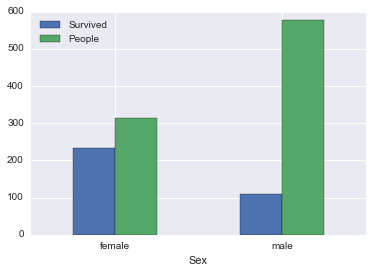
Now that you have a rough understanding of what each feature entail. Let’s first start by exploring how gender is related to the overall survival rate.
In [4]:
survived_filter = ~union.Survived.isnull()

survived_by_sex = union[survived_filter] [['Sex', 'Survived']].groupby('Sex').sum()

survived_by_sex['People'] = union[survived_filter].groupby('Sex').count().Survived

survived_by_sex['PctSurvived'] = survived_by_sex.Survived / survived_by_sex.People

survived_by_sex| Survived | People | PctSurvived | |
|---|---|---|---|
| Sex | |||
| female | 233.0 | 314 | 0.742038 |
| male | 109.0 | 577 | 0.188908 |
This makes sense, Titanic’s evacuation procedure had a women and children first policy. So, vast majority of the women were led into a safety boat.
In [5]:
survived_by_sex[['Survived', 'People']].plot(kind='bar', rot=0)<matplotlib.axes._subplots.AxesSubplot at 0x117a3f668>
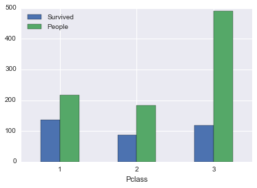
Passenger Class
What about survivial with respect to each passenger class (Pclass)? Do people with higher social class tend live through the catastrophe?
In [6]:
survived_by_pclass = union[survived_filter][['Pclass', 'Survived']].groupby('Pclass').sum()

survived_by_pclass['People'] = union[survived_filter].groupby('Pclass').count().Survived

survived_by_pclass['PctSurvived'] = survived_by_pclass.Survived / survived_by_pclass.People

survived_by_pclass| Survived | People | PctSurvived | |
|---|---|---|---|
| Pclass | |||
| 1 | 136.0 | 216 | 0.629630 |
| 2 | 87.0 | 184 | 0.472826 |
| 3 | 119.0 | 491 | 0.242363 |
So people in higher pclasses do have higher survivability. It’s hard to say why without digging into the details, maybe it’s the way they’re dressed, the way they conduct themselves during emergencies, better connected, or a higher percentage of women (which we found from earlier exploration that females tend to be led into life boats easier). All these questions are things we want to keep in mind.
In [7]:
survived_by_pclass[['Survived', 'People']].plot(kind='bar', rot=0)<matplotlib.axes._subplots.AxesSubplot at 0x117b91390>
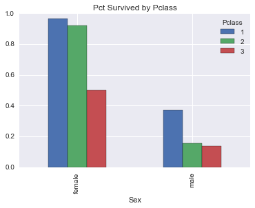
How about if we separated social class and gender, how does our survival rate look?
In [8]:
survived_by_pclass_sex = union[survived_filter].groupby(['Sex', 'Pclass']) \
    .apply(lambda x: x.Survived.sum() / len(x)) \
    .unstack()

survived_by_pclass_sex| Pclass | 1 | 2 | 3 |
|---|---|---|---|
| Sex | |||
| female | 0.968085 | 0.921053 | 0.500000 |
| male | 0.368852 | 0.157407 | 0.135447 |
Looks between passenger classes, male in higher classes gets the biggest survivability boost. And let’s graph this for some visuals.
In [9]:
survived_by_pclass_sex.plot(kind='bar', title='Pct Survived by Pclass')<matplotlib.axes._subplots.AxesSubplot at 0x117ba59e8>
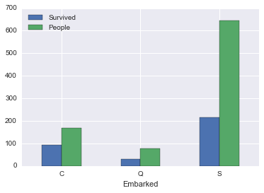
Port of Embarkment
In [10]:
survived_by_embarked = union[survived_filter][['Embarked', 'Survived']].groupby('Embarked').sum()

survived_by_embarked['People'] = union[survived_filter][['Embarked', 'Survived']].groupby('Embarked').count()

survived_by_embarked['PctSurvived'] = survived_by_embarked.Survived/survived_by_embarked.People

survived_by_embarked| Survived | People | PctSurvived | |
|---|---|---|---|
| Embarked | |||
| C | 93.0 | 168 | 0.553571 |
| Q | 30.0 | 77 | 0.389610 |
| S | 217.0 | 644 | 0.336957 |
So embarking at port C gives a higher survivability rate, I wonder why.
In [11]:
survived_by_embarked[['Survived', 'People']].plot(kind='bar', rot=0)<matplotlib.axes._subplots.AxesSubplot at 0x117ae16d8>
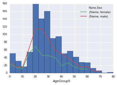
Age
So was the Titanic filled with kids? or seniors?
I’ve grouped people into buckets of 5 years, starting with age 0.
In [12]:
union.loc[~union.Age.isnull(), 'AgeGroup5'] = union.Age.dropna().apply(lambda x: int(x/5)*5)

ax = union.Age.hist(bins=len(union.AgeGroup5.unique()))
union[['Sex', 'AgeGroup5', 'Name']].groupby(['AgeGroup5', 'Sex']).count().unstack('Sex').plot(ax=ax)
<matplotlib.axes._subplots.AxesSubplot at 0x117a6d630>
We can get a bit more granular, let’s break down the ages by passenger classes.
In [13]:
fig, axes = plt.subplots(1, 3, figsize=(16,4))

for i in range(3):
    union[union.Pclass == i+1]['Age'].hist(ax = axes[i])
    axes[i].set_title("Pclass {} Age Distribution".format(i+1))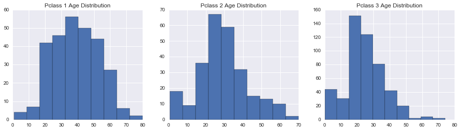
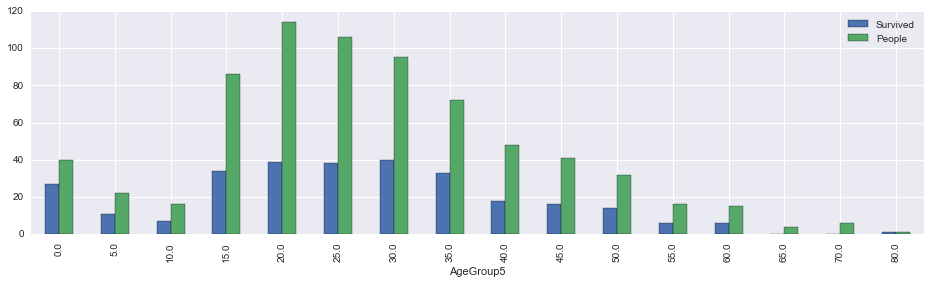
So we think that kids, like females, were given priority during the evacuation. Let’s check if this this true.
In [14]:
survived_by_agegroup5 = union[~union.Survived.isnull()][['AgeGroup5', 'Survived']].groupby('AgeGroup5').sum()

survived_by_agegroup5['People'] = union[~union.Survived.isnull()][['AgeGroup5', 'Survived']].groupby('AgeGroup5').count()

survived_by_agegroup5['PctSurvived'] = survived_by_agegroup5.Survived/survived_by_agegroup5.People

survived_by_agegroup5.head()| Survived | People | PctSurvived | |
|---|---|---|---|
| AgeGroup5 | |||
| 0.0 | 27.0 | 40 | 0.675000 |
| 5.0 | 11.0 | 22 | 0.500000 |
| 10.0 | 7.0 | 16 | 0.437500 |
| 15.0 | 34.0 | 86 | 0.395349 |
| 20.0 | 39.0 | 114 | 0.342105 |
In [15]:
survived_by_agegroup5[['Survived', 'People']].plot(kind='bar', figsize=(16,4))<matplotlib.axes._subplots.AxesSubplot at 0x11aca5748>
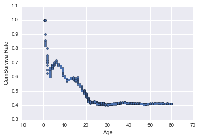
Running survival rate
Thought I’d try something different by plotting the cumulative survival rate from age 0, to see how it drops off as you get older.
In [16]:
survived_by_age = union[~union.Survived.isnull()][train.Age <= 60][['Age', 'Survived']].sort_values('Age')

survived_by_age['CumSurvived'] = survived_by_age.Survived.cumsum()

survived_by_age['CumCount'] = [x+1 for x in range(len(survived_by_age))]

survived_by_age['CumSurvivalRate'] = survived_by_age.CumSurvived / survived_by_age.CumCount

survived_by_age.plot(kind='scatter', x='Age', y='CumSurvivalRate')
<matplotlib.axes._subplots.AxesSubplot at 0x11b109978>
In [17]:
survived_by_age[(survived_by_age.Age >= 5) & (survived_by_age.Age <= 8)].head()| Age | Survived | CumSurvived | CumCount | CumSurvivalRate | |
|---|---|---|---|---|---|
| 233 | 5.0 | 1.0 | 28.0 | 41 | 0.682927 |
| 58 | 5.0 | 1.0 | 29.0 | 42 | 0.690476 |
| 777 | 5.0 | 1.0 | 30.0 | 43 | 0.697674 |
| 448 | 5.0 | 1.0 | 31.0 | 44 | 0.704545 |
| 751 | 6.0 | 1.0 | 32.0 | 45 | 0.711111 |
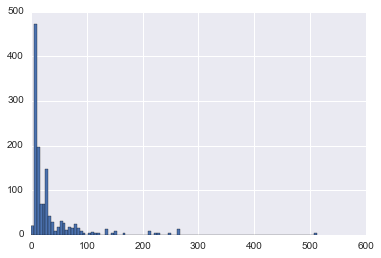
Fare
Fare by default is like a proxy for passenger class. The more expensive the fare, the wealthier you are.
Anyways, let’s visual what the actual fare price distribution looks like.
In [18]:
union.Fare.hist(bins=100)<matplotlib.axes._subplots.AxesSubplot at 0x11b324ac8>
In [19]:
union[['Pclass', 'Fare']].groupby('Pclass').describe().unstack()| Fare | ||||||||
|---|---|---|---|---|---|---|---|---|
| count | mean | std | min | 25% | 50% | 75% | max | |
| Pclass | ||||||||
| 1 | 323.0 | 87.508992 | 80.447178 | 0.0 | 30.6958 | 60.0000 | 107.6625 | 512.3292 |
| 2 | 277.0 | 21.179196 | 13.607122 | 0.0 | 13.0000 | 15.0458 | 26.0000 | 73.5000 |
| 3 | 708.0 | 13.302889 | 11.494358 | 0.0 | 7.7500 | 8.0500 | 15.2458 | 69.5500 |
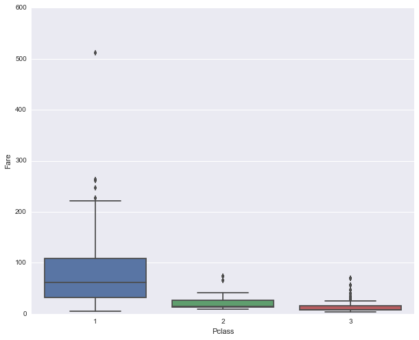
We need to come back and revisit Fare, since there are fares prices at $0 or null.
In [20]:
fare_invalid_filter = (union.Fare.isnull()) | (union.Fare < 1)
len(union[fare_invalid_filter])
18
In [21]:
fig, ax = plt.subplots(figsize=(10,8))

sns.boxplot(data=union[~fare_invalid_filter], x='Pclass', y='Fare', ax=ax)
<matplotlib.axes._subplots.AxesSubplot at 0x11b722f98>
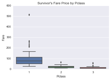
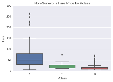
Let’s see if there’s a relationshp between fare price and those who has survived
In [22]:
union[['Pclass', 'Fare']][(~fare_invalid_filter) & (union.Survived == 1)].groupby('Pclass').describe().unstack()| Fare | ||||||||
|---|---|---|---|---|---|---|---|---|
| count | mean | std | min | 25% | 50% | 75% | max | |
| Pclass | ||||||||
| 1 | 136.0 | 95.608029 | 85.286820 | 25.9292 | 50.98545 | 77.9583 | 111.481225 | 512.3292 |
| 2 | 87.0 | 22.055700 | 10.853502 | 10.5000 | 13.00000 | 21.0000 | 26.250000 | 65.0000 |
| 3 | 118.0 | 13.810946 | 10.663057 | 6.9750 | 7.77500 | 8.5896 | 15.887500 | 56.4958 |
In [23]:
union[['Pclass', 'Fare']][(~fare_invalid_filter) & (union.Survived == 0)].groupby('Pclass').describe().unstack()| Fare | ||||||||
|---|---|---|---|---|---|---|---|---|
| count | mean | std | min | 25% | 50% | 75% | max | |
| Pclass | ||||||||
| 1 | 75.0 | 68.996275 | 60.224407 | 5.0000 | 29.7000 | 50.00 | 79.2000 | 263.00 |
| 2 | 91.0 | 20.692262 | 14.938248 | 10.5000 | 12.9375 | 13.00 | 26.0000 | 73.50 |
| 3 | 369.0 | 13.780497 | 12.104365 | 4.0125 | 7.7500 | 8.05 | 15.2458 | 69.55 |
In [24]:
sns.boxplot(data=union[(~fare_invalid_filter) & (union.Survived == 1)], x='Pclass', y='Fare')
plt.title("Survivor's Fare Price by Pclass")

plt.figure()
sns.boxplot(data=union[(~fare_invalid_filter) & (union.Survived == 0)], x='Pclass', y='Fare')
plt.title("Non-Survivor's Fare Price by Pclass")
<matplotlib.text.Text at 0x11bdfb860>
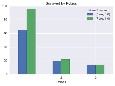
Percentage of people surivived by pclass
And not surpringly, people in better passenger classes had higher surivival rate
In [25]:
survived_by_fare_pclass = union[~union.Survived.isnull()][['Fare', 'Survived', 'Pclass']].groupby(['Pclass', 'Survived']).mean().unstack('Survived')
survived_by_fare_pclass.plot(kind='bar', rot=0)
plt.title('Survived by Pclass')
<matplotlib.text.Text at 0x11beb5240>
Cabin
There’s a lot of missing values in the cabin feature, but let’s check it out anyways. We would think that the closer your cabin is to the life rafts, the better your chances are.
First, we need to strip out the cabin number in the cabin column.
In [26]:
# Define cabin class
union.loc[~union.Cabin.isnull(), 'CabinClass'] = union.Cabin.dropna().str[0]
In [27]:
cabinclass = union[~union.Survived.isnull()][['CabinClass', 'Survived']].groupby('CabinClass').sum()
cabinclass['People'] = union[~union.Survived.isnull()].groupby('CabinClass').count().Survived
cabinclass['PctSurvived'] = cabinclass.Survived / cabinclass.People
cabinclass['AvgFare'] = union[(~union.Survived.isnull()) & (~fare_invalid_filter)].groupby('CabinClass').mean().Fare
cabinclass['AvgAge'] = union[~union.Survived.isnull()].groupby('CabinClass').mean().Age
cabinclass['PctFemaleInCabin'] = union[~union.Survived.isnull()].groupby('CabinClass').apply(lambda x: len(x[x.Sex == 'female']) / len(x))

cabinclass| Survived | People | PctSurvived | AvgFare | AvgAge | PctFemaleInCabin | |
|---|---|---|---|---|---|---|
| CabinClass | ||||||
| A | 7.0 | 15 | 0.466667 | 42.454164 | 44.833333 | 0.066667 |
| B | 35.0 | 47 | 0.744681 | 118.550464 | 34.955556 | 0.574468 |
| C | 35.0 | 59 | 0.593220 | 100.151341 | 36.086667 | 0.457627 |
| D | 25.0 | 33 | 0.757576 | 57.244576 | 39.032258 | 0.545455 |
| E | 24.0 | 32 | 0.750000 | 46.026694 | 38.116667 | 0.468750 |
| F | 8.0 | 13 | 0.615385 | 18.696792 | 19.954545 | 0.384615 |
| G | 2.0 | 4 | 0.500000 | 13.581250 | 14.750000 | 1.000000 |
| T | 0.0 | 1 | 0.000000 | 35.500000 | 45.000000 | 0.000000 |
Weird how there’s a single person in cabin T …
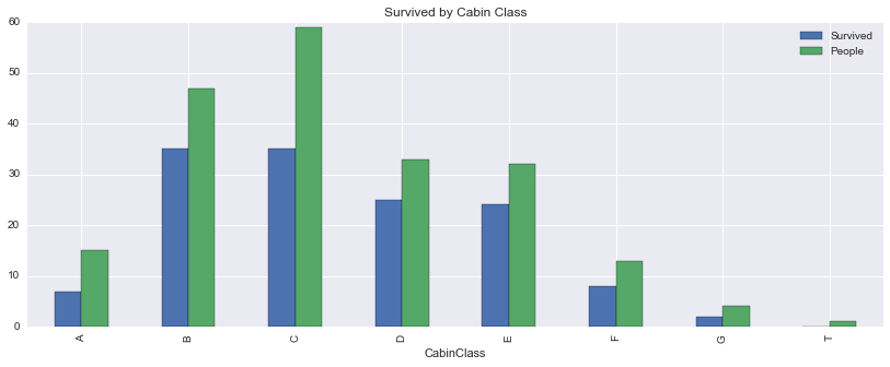
More visualizations by cabin class!
In [28]:
cabinclass[['Survived', 'People']].plot(kind='bar', figsize=(14,5), title='Survived by Cabin Class')<matplotlib.axes._subplots.AxesSubplot at 0x11bea8da0>
Feature Engineering
Alright, the fun begins. Now we need to think of new features to add into our classifier, what can we deduce from the raw components we have already examined earlier?
One quick way of picking out the features with missing values is to look at the non-null count from the describe() function. Also, we can visually inspect the quantiles of each feature to see if it makes logically sense. For example, why does the Fare feature has a min price of 0?
In [29]:
union.describe()| Age | Fare | Parch | PassengerId | Pclass | SibSp | Survived | AgeGroup5 | |
|---|---|---|---|---|---|---|---|---|
| count | 1046.000000 | 1308.000000 | 1309.000000 | 1309.000000 | 1309.000000 | 1309.000000 | 891.000000 | 1046.00000 |
| mean | 29.881138 | 33.295479 | 0.385027 | 655.000000 | 2.294882 | 0.498854 | 0.383838 | 27.90631 |
| std | 14.413493 | 51.758668 | 0.865560 | 378.020061 | 0.837836 | 1.041658 | 0.486592 | 14.60369 |
| min | 0.170000 | 0.000000 | 0.000000 | 1.000000 | 1.000000 | 0.000000 | 0.000000 | 0.00000 |
| 25% | 21.000000 | 7.895800 | 0.000000 | 328.000000 | 2.000000 | 0.000000 | 0.000000 | 20.00000 |
| 50% | 28.000000 | 14.454200 | 0.000000 | 655.000000 | 3.000000 | 0.000000 | 0.000000 | 25.00000 |
| 75% | 39.000000 | 31.275000 | 0.000000 | 982.000000 | 3.000000 | 1.000000 | 1.000000 | 35.00000 |
| max | 80.000000 | 512.329200 | 9.000000 | 1309.000000 | 3.000000 | 8.000000 | 1.000000 | 80.00000 |
Extracting Titles from Name
Name has a wealth of string information that we can take advantage of. Notice how each person has a prefix, maybe we can extract this out and use it to predict the age of the person if it’s missing.
In [30]:
union['Title'] = union.Name.apply(lambda x: (x.split(',')[1]).split('.')[0][1:])
union[['Age','Title']].groupby('Title').describe().unstack()| Age | ||||||||
|---|---|---|---|---|---|---|---|---|
| count | mean | std | min | 25% | 50% | 75% | max | |
| Title | ||||||||
| Capt | 1.0 | 70.000000 | NaN | 70.00 | 70.00 | 70.0 | 70.00 | 70.0 |
| Col | 4.0 | 54.000000 | 5.477226 | 47.00 | 51.50 | 54.5 | 57.00 | 60.0 |
| Don | 1.0 | 40.000000 | NaN | 40.00 | 40.00 | 40.0 | 40.00 | 40.0 |
| Dona | 1.0 | 39.000000 | NaN | 39.00 | 39.00 | 39.0 | 39.00 | 39.0 |
| Dr | 7.0 | 43.571429 | 11.731115 | 23.00 | 38.00 | 49.0 | 51.50 | 54.0 |
| Jonkheer | 1.0 | 38.000000 | NaN | 38.00 | 38.00 | 38.0 | 38.00 | 38.0 |
| Lady | 1.0 | 48.000000 | NaN | 48.00 | 48.00 | 48.0 | 48.00 | 48.0 |
| Major | 2.0 | 48.500000 | 4.949747 | 45.00 | 46.75 | 48.5 | 50.25 | 52.0 |
| Master | 53.0 | 5.482642 | 4.161554 | 0.33 | 2.00 | 4.0 | 9.00 | 14.5 |
| Miss | 210.0 | 21.774238 | 12.249077 | 0.17 | 15.00 | 22.0 | 30.00 | 63.0 |
| Mlle | 2.0 | 24.000000 | 0.000000 | 24.00 | 24.00 | 24.0 | 24.00 | 24.0 |
| Mme | 1.0 | 24.000000 | NaN | 24.00 | 24.00 | 24.0 | 24.00 | 24.0 |
| Mr | 581.0 | 32.252151 | 12.422089 | 11.00 | 23.00 | 29.0 | 39.00 | 80.0 |
| Mrs | 170.0 | 36.994118 | 12.901767 | 14.00 | 27.00 | 35.5 | 46.50 | 76.0 |
| Ms | 1.0 | 28.000000 | NaN | 28.00 | 28.00 | 28.0 | 28.00 | 28.0 |
| Rev | 8.0 | 41.250000 | 12.020815 | 27.00 | 29.50 | 41.5 | 51.75 | 57.0 |
| Sir | 1.0 | 49.000000 | NaN | 49.00 | 49.00 | 49.0 | 49.00 | 49.0 |
| the Countess | 1.0 | 33.000000 | NaN | 33.00 | 33.00 | 33.0 | 33.00 | 33.0 |
Are some titles tend to dominate in one gender?
In [31]:
union[['Sex','Title','Survived']].groupby(['Title','Sex']).sum().unstack('Sex')| Survived | ||
|---|---|---|
| Sex | female | male |
| Title | ||
| Capt | NaN | 0.0 |
| Col | NaN | 1.0 |
| Don | NaN | 0.0 |
| Dona | NaN | NaN |
| Dr | 1.0 | 2.0 |
| Jonkheer | NaN | 0.0 |
| Lady | 1.0 | NaN |
| Major | NaN | 1.0 |
| Master | NaN | 23.0 |
| Miss | 127.0 | NaN |
| Mlle | 2.0 | NaN |
| Mme | 1.0 | NaN |
| Mr | NaN | 81.0 |
| Mrs | 99.0 | NaN |
| Ms | 1.0 | NaN |
| Rev | NaN | 0.0 |
| Sir | NaN | 1.0 |
| the Countess | 1.0 | NaN |
Working with all these different kinds of titles can overfit our data, let’s try classifying the less frequent titles into either Mr, Mrs, Miss, Master and Officer. The goal is to come up with the fewest number of unique titles that does not give us overlapping age ranges.
In [32]:
def title_mapping(x):
    #if x in set(['Capt', 'Col', 'Don', 'Major', 'Rev', 'Sir', 'Jonkheer']):
    if x.Title in set(['Don', 'Rev', 'Sir', 'Jonkheer']):
        return 'Mr'
    elif x.Title in set(['Lady', 'the Countess']):
        return 'Mrs'
    elif x.Title in set(['Mlle', 'Mme', 'Dona', 'Ms']):
        return "Miss"
    elif x.Title in set(['Major', 'Col', 'Capt']):
        return "Officer"
    elif x.Title == 'Dr' and x.Sex == 'female':
        return 'Mrs'
    elif x.Title == 'Dr' and x.Sex == 'male':
        return 'Mr'
    else:
        return x.Title

union.Title = union.apply(title_mapping, axis=1)
union.Title.unique()
array(['Mr', 'Mrs', 'Miss', 'Master', 'Officer'], dtype=object)
Let see how well we have separated out the age groups by title.
In [33]:
union[['Age', 'Title']].groupby('Title').describe().unstack()| Age | ||||||||
|---|---|---|---|---|---|---|---|---|
| count | mean | std | min | 25% | 50% | 75% | max | |
| Title | ||||||||
| Master | 53.0 | 5.482642 | 4.161554 | 0.33 | 2.0 | 4.0 | 9.0 | 14.5 |
| Miss | 215.0 | 21.914372 | 12.171758 | 0.17 | 15.5 | 22.0 | 30.0 | 63.0 |
| Mr | 598.0 | 32.527592 | 12.476329 | 11.00 | 23.0 | 30.0 | 40.0 | 80.0 |
| Mrs | 173.0 | 37.104046 | 12.852049 | 14.00 | 27.0 | 36.0 | 47.0 | 76.0 |
| Officer | 7.0 | 54.714286 | 8.440266 | 45.00 | 49.5 | 53.0 | 58.0 | 70.0 |
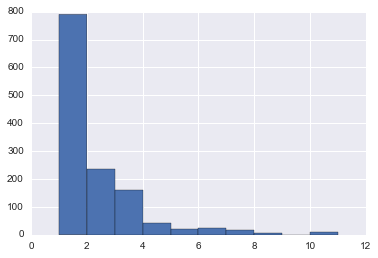
Family Size
In [34]:
union['FamilySize'] = union.Parch + union.SibSp + 1
union[['Parch', 'SibSp', 'FamilySize']][union.FamilySize > 3].head(3)| Parch | SibSp | FamilySize | |
|---|---|---|---|
| 7 | 1 | 3 | 5 |
| 13 | 5 | 1 | 7 |
| 16 | 1 | 4 | 6 |
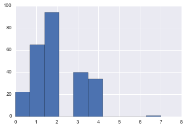
In [35]:
union.FamilySize.hist()<matplotlib.axes._subplots.AxesSubplot at 0x11c347550>
In [36]:
def family_size_bucket(x):
    if x <= 1:
        return "Single"
    elif x <= 3:
        return "Small"
    elif x <= 5:
        return "Median"
    else:
        return "Large"

union['FamilySizeBucket'] = union.FamilySize.apply(family_size_bucket)
Lone Travellers
In [37]:
union['Alone'] = union.FamilySize.apply(lambda x: 1 if x == 1 else 0)In [38]:
survived_by_alone = union[~union.Survived.isnull()][['Survived', 'Alone']].groupby('Alone').sum()
survived_by_alone['People'] = union[~union.Survived.isnull()][['Survived', 'Alone']].groupby('Alone').count()
survived_by_alone['PctSurvived'] = survived_by_alone.Survived / survived_by_alone.People
survived_by_alone| Survived | People | PctSurvived | |
|---|---|---|---|
| Alone | |||
| 0 | 179.0 | 354 | 0.505650 |
| 1 | 163.0 | 537 | 0.303538 |
Family Name
Extract out the family names
In [39]:
union['FamilyName'] = union.Name.apply(lambda x: x.split(",")[0])In [40]:
survived_by_family_name = union[['Survived', 'FamilyName']].groupby('FamilyName').sum()
survived_by_family_name['FamilySize'] = union[['FamilySize', 'FamilyName']].groupby('FamilyName').max()

survived_by_family_name.head()| Survived | FamilySize | |
|---|---|---|
| FamilyName | ||
| Abbing | 0.0 | 1 |
| Abbott | 1.0 | 3 |
| Abelseth | NaN | 1 |
| Abelson | 1.0 | 2 |
| Abrahamsson | NaN | 1 |
Are families more likely to survive?
In [41]:
survived_by_family_size = survived_by_family_name.groupby('FamilySize').sum()
survived_by_family_size['FamilyCount'] = survived_by_family_name.groupby('FamilySize').count()
survived_by_family_size['PeopleInFamily'] = survived_by_family_size.FamilyCount * survived_by_family_size.index
survived_by_family_size['PctSurvived'] = survived_by_family_size.Survived / survived_by_family_size.PeopleInFamily

survived_by_family_size| Survived | FamilyCount | PeopleInFamily | PctSurvived | |
|---|---|---|---|---|
| FamilySize | ||||
| 1 | 153.0 | 475 | 475 | 0.322105 |
| 2 | 89.0 | 104 | 208 | 0.427885 |
| 3 | 65.0 | 59 | 177 | 0.367232 |
| 4 | 21.0 | 14 | 56 | 0.375000 |
| 5 | 4.0 | 6 | 30 | 0.133333 |
| 6 | 5.0 | 5 | 30 | 0.166667 |
| 7 | 5.0 | 2 | 14 | 0.357143 |
| 8 | 0.0 | 1 | 8 | 0.000000 |
| 11 | 0.0 | 1 | 11 | 0.000000 |
Impute Missing Values
Label Encoding
Categorical columns needs to be mapped to ints for some classifiers to work. We’ll use the sklearn.preprocessing.LableEncoder() to help us with this.
In [42]:
encoder_list = ['Sex', 'Pclass', 'Title','FamilyName', 'FamilySizeBucket']
encoder = []

for i, e in enumerate(encoder_list):
    print(i,e)
    encoder.append(sklearn.preprocessing.LabelEncoder())
    union['{}Encoding'.format(e)] = encoder[i].fit_transform(union[e])
0 Sex
1 Pclass
2 Title
3 FamilyName
4 FamilySizeBucket
Embarked
This is a bit of an overkill, but we have 1 passenger missing her port of emarkment. Simple analysis would’ve sufficed, but let’s go the whole nine yards anyways for completeness’ sake.
In [43]:
embarked_features = ['Age', 'Cabin', 'Embarked', 'Fare', 'Name', 'Parch', 'PassengerId',
       'Pclass', 'Sex', 'SibSp', 'Survived', 'Ticket',
       'CabinClass', 'Title', 'FamilySize', 'Alone', 'FamilyName']
In [44]:
embarked_breakdown = union.loc[union.Pclass == 1, ['Pclass', 'Embarked', 'Survived']].groupby(['Pclass', 'Embarked']).sum()
embarked_breakdown['Count'] = union.loc[union.Pclass == 1, ['Pclass', 'Embarked', 'Survived']].groupby(['Pclass', 'Embarked']).count()
embarked_breakdown['AvgFare'] = union.loc[union.Pclass == 1, ['Pclass', 'Embarked', 'Fare']].groupby(['Pclass', 'Embarked']).mean().Fare
embarked_breakdown['AvgAge'] = union.loc[union.Pclass == 1, ['Pclass', 'Embarked', 'Age']].groupby(['Pclass', 'Embarked']).mean().Age

embarked_breakdown| Survived | Count | AvgFare | AvgAge | ||
|---|---|---|---|---|---|
| Pclass | Embarked | ||||
| 1 | C | 59.0 | 85 | 106.845330 | 39.062500 |
| Q | 1.0 | 2 | 90.000000 | 38.000000 | |
| S | 74.0 | 127 | 72.148094 | 39.121987 |
In [45]:
union.loc[union.Pclass == 1, ['Pclass', 'Embarked', 'CabinClass', 'Survived']].groupby(['Pclass', 'Embarked', 'CabinClass']).count()| Survived | |||
|---|---|---|---|
| Pclass | Embarked | CabinClass | |
| 1 | C | A | 7 |
| B | 22 | ||
| C | 21 | ||
| D | 11 | ||
| E | 5 | ||
| Q | C | 2 | |
| S | A | 8 | |
| B | 23 | ||
| C | 36 | ||
| D | 18 | ||
| E | 20 | ||
| T | 1 |
In [46]:
union.loc[union.Pclass == 1, ['Pclass', 'Embarked', 'Sex', 'Survived']].groupby(['Pclass', 'Embarked', 'Sex']).count()| Survived | |||
|---|---|---|---|
| Pclass | Embarked | Sex | |
| 1 | C | female | 43 |
| male | 42 | ||
| Q | female | 1 | |
| male | 1 | ||
| S | female | 48 | |
| male | 79 |
For imputation, let’s train a k nearest neighbor classifer to figure out which port of embarkment you’re from.
In [47]:
embarked_features = ['Parch', 'PclassEncoding', 'SexEncoding', 'SibSp',
                    'TitleEncoding', 'FamilySize', 'Alone', 'FamilyNameEncoding', 'FamilySizeBucketEncoding']
In [48]:
params = {'n_neighbors' : [5, 10, 15, 30, 50, 100, 200]}

clf_embarked = sklearn.grid_search.GridSearchCV(sklearn.neighbors.KNeighborsClassifier(), params, cv=5, n_jobs=4)
clf_embarked.fit(union[~union.Embarked.isnull()][embarked_features], union[~union.Embarked.isnull()].Embarked)

clf_embarked.predict(union[union.Embarked.isnull()][embarked_features])
array(['S', 'S'], dtype=object)
KNN tells us that our passenger with no port of embarkment probably boarded from “S”, let’s fill that in.
In [49]:
union.loc[union.Embarked.isnull(), 'Embarked'] = 'S'Let’s run our encoder code again on Embarked.
In [50]:
encoder_list = ['Embarked']
encoder = []

for i, e in enumerate(encoder_list):
    print(i,e)
    encoder.append(sklearn.preprocessing.LabelEncoder())
    union['{}Encoding'.format(e)] = encoder[i].fit_transform(union[e])
0 Embarked
Ticket
There’s a bit of judgemenet call in this one. The goal is to bucket the ticket strings into various classes. After going through all the labels, you slowly start to see some patterns.
In [51]:
def ticket_cleaning(x):
    ticket = x.split(' ')[0].replace('.', '').replace(r'/', '')
    if ticket.isdigit():
        return 'Integer_Group'
    elif 'TON' in ticket:
        return 'STON_Group'
    elif ticket[0] == 'A':
        return 'A_Group'
    elif ticket[0] == 'C':
        return 'C_Group'
    elif ticket[0] == 'F':
        return 'F_Group'
    elif ticket[0] == 'L':
        return 'L_Group'
    elif ticket[:2] == 'SC' or ticket == 'SOC':
        return 'SC_Group'
    elif ticket[:3] == 'SOP' or ticket == 'SP' or ticket == 'SWPP':
        return 'SP_Group'
    elif ticket[0] == 'P':
        return 'P_Group'
    elif ticket[0] == 'W':
        return 'W_Group'

    return ticket

union['TicketGroup'] = union['Ticket'].apply(ticket_cleaning)
union[['TicketGroup', 'Survived']].groupby('TicketGroup').count()| Survived | |
|---|---|
| TicketGroup | |
| A_Group | 29 |
| C_Group | 46 |
| F_Group | 7 |
| Integer_Group | 661 |
| L_Group | 4 |
| P_Group | 65 |
| SC_Group | 23 |
| SP_Group | 7 |
| STON_Group | 36 |
| W_Group | 13 |
In [52]:
encoder_list = ['TicketGroup']
encoder = []

for i, e in enumerate(encoder_list):
    print(i,e)
    encoder.append(sklearn.preprocessing.LabelEncoder())
    union['{}Encoding'.format(e)] = encoder[i].fit_transform(union[e])
0 TicketGroup
Impute Age
Yay, if you actually read this far. Age is a very important factor in predicting survivability, so let’s take in all the raw and engineered features and fill in the blanks for our passengers.
In [53]:
age_features = ['EmbarkedEncoding', 'SexEncoding', 'PclassEncoding',
                'Alone', 'SibSp', 'Parch', 'FamilySize', 'TitleEncoding', 'TicketGroupEncoding']

#clf_age = sklearn.linear_model.RidgeCV(alphas=[0.1, 0.5, 1, 3, 10])
#clf_age = sklearn.linear_model.RidgeCV(alphas=[0.1, 0.5, 1, 3, 10])

params = {'n_neighbors' : [5, 10, 15, 30, 50, 100, 200]}

clf_age = sklearn.grid_search.GridSearchCV(sklearn.neighbors.KNeighborsRegressor(), params, cv=5, n_jobs=4)
clf_age.fit(union[~union.Age.isnull()][age_features], union[~union.Age.isnull()].Age)
print(clf_age.best_params_)
{'n_neighbors': 15}
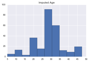
In [54]:
pd.Series(clf_age.predict(union[union.Age.isnull()][age_features])).hist()
plt.title('Imputed Age')
<matplotlib.text.Text at 0x11be70978>
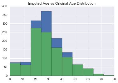
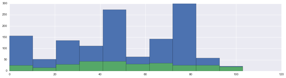
Now that we’ve trained our classifier, how does the new imputed age distribution look like compared to the old one?
In [55]:
union['ImputedAge'] = union.Age
union.loc[(union.Age.isnull()), 'ImputedAge'] = clf_age.predict(union[(union.Age.isnull())][age_features])

union['ImputedAge'].hist()
union['Age'].hist()
plt.title('Imputed Age vs Original Age Distribution')
<matplotlib.text.Text at 0x11bda60f0>
Impute Fare
In [56]:
union[['Pclass', 'Fare']].groupby('Pclass').describe().unstack()| Fare | ||||||||
|---|---|---|---|---|---|---|---|---|
| count | mean | std | min | 25% | 50% | 75% | max | |
| Pclass | ||||||||
| 1 | 323.0 | 87.508992 | 80.447178 | 0.0 | 30.6958 | 60.0000 | 107.6625 | 512.3292 |
| 2 | 277.0 | 21.179196 | 13.607122 | 0.0 | 13.0000 | 15.0458 | 26.0000 | 73.5000 |
| 3 | 708.0 | 13.302889 | 11.494358 | 0.0 | 7.7500 | 8.0500 | 15.2458 | 69.5500 |
In [57]:
fig, axes = plt.subplots(1, 3, figsize=(16, 4))

#union[['Pclass', 'Fare']]
for i, pclass in enumerate(np.sort(union.Pclass.unique())):
    union[union.Pclass == pclass].Fare.hist(ax=axes[i])
    axes[i].set_title('Fare Distribution for Pclass={}'.format(pclass))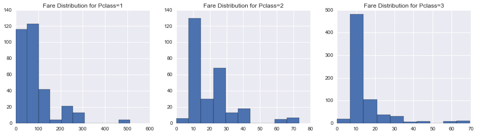
In [58]:
fare_features_knn = ['EmbarkedEncoding', 'SexEncoding', 'PclassEncoding',
                'Alone', 'SibSp', 'Parch', 'FamilySize', 'TitleEncoding',
                 'ImputedAge', 'TicketGroupEncoding']

fare_features_ridge = ['EmbarkedEncoding', 'PclassEncoding',
                'Alone', 'SibSp', 'Parch', 'ImputedAge']

fare_features = fare_features_knn

params = {'n_neighbors' : [2, 4, 7, 10, 15, 30, 50, 100, 200]}
clf_fare = sklearn.grid_search.GridSearchCV(sklearn.neighbors.KNeighborsRegressor(), params, cv=5, n_jobs=4)

#clf_fare = sklearn.linear_model.RidgeCV(alphas=[0.1, 0.5, 1, 3, 10])

clf_fare.fit(union[~union.Fare.isnull()][fare_features], union[~union.Fare.isnull()].Fare)
#print(clf_fare.best_params_)
GridSearchCV(cv=5, error_score='raise',
estimator=KNeighborsRegressor(algorithm='auto', leaf_size=30, metric='minkowski',
metric_params=None, n_jobs=1, n_neighbors=5, p=2,
weights='uniform'),
fit_params={}, iid=True, n_jobs=4,
param_grid={'n_neighbors': [2, 4, 7, 10, 15, 30, 50, 100, 200]},
pre_dispatch='2*n_jobs', refit=True, scoring=None, verbose=0)
In [59]:
union.loc[((union.Fare.isnull()) | (union.Fare <= 0)), ['Pclass', 'Fare']].groupby('Pclass').count()| Fare | |
|---|---|
| Pclass | |
| 1 | 7 |
| 2 | 6 |
| 3 | 4 |
In [60]:
union['ImputedFare'] = union.Fare

union.loc[union.Fare.isnull(), 'ImputedFare'] = clf_fare.predict(union[union.Fare.isnull()][fare_features])
In [61]:
fig, axes = plt.subplots(1, 3, figsize=(16, 4))

for i, pclass in enumerate(np.sort(union.Pclass.unique())):
    null_fare_pclass_filter = ((union.Pclass == pclass) & ((union.Fare.isnull()) | (union.Fare <= 0)))
    pd.Series(clf_fare.predict(union[null_fare_pclass_filter][fare_features])).hist(ax=axes[i])
    axes[i].set_title('Imputed Fare for Pclass={}'.format(pclass))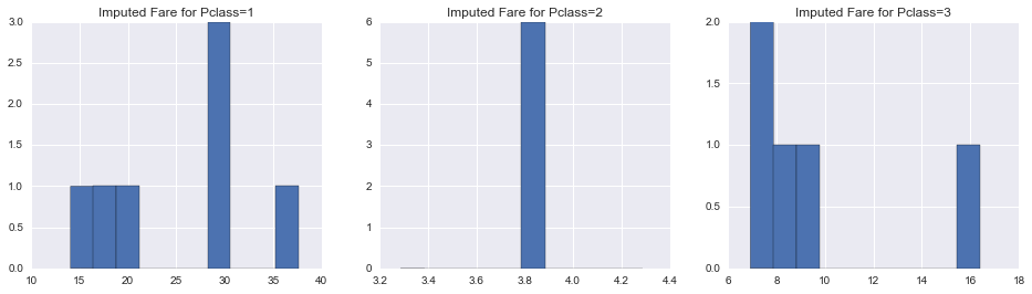
In [62]:
union[union.Fare.isnull() | union.Fare <= 0][fare_features].head()| EmbarkedEncoding | SexEncoding | PclassEncoding | Alone | SibSp | Parch | FamilySize | TitleEncoding | ImputedAge | TicketGroupEncoding | |
|---|---|---|---|---|---|---|---|---|---|---|
| 179 | 2 | 1 | 2 | 1 | 0 | 0 | 1 | 2 | 36.0 | 4 |
| 263 | 2 | 1 | 0 | 1 | 0 | 0 | 1 | 2 | 40.0 | 3 |
| 271 | 2 | 1 | 2 | 1 | 0 | 0 | 1 | 2 | 25.0 | 4 |
| 277 | 2 | 1 | 1 | 1 | 0 | 0 | 1 | 2 | 32.0 | 3 |
| 302 | 2 | 1 | 2 | 1 | 0 | 0 | 1 | 2 | 19.0 | 4 |
In [63]:
fig, axes = plt.subplots(1, 3, figsize=(16, 4))

for i, pclass in enumerate(np.sort(union.Pclass.unique())):
    union[union.Pclass == pclass].ImputedFare.hist(ax=axes[i])
    union[union.Pclass == pclass].Fare.hist(ax=axes[i])
    axes[i].set_title('Imputed Fare Distribution for Pclass={}'.format(pclass))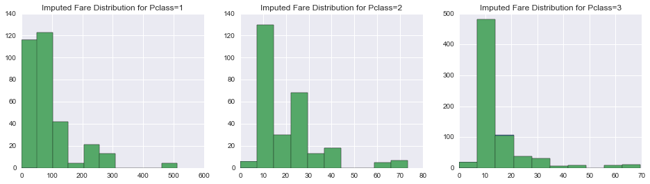
Mother
“Mother and children first”, so I think that’s what they’d say as the Titanic is sinking. Let’s try to identify the mothers using the passenger’s gender, age, title, and whether if she has a child.
In [64]:
union['Mother'] = union.apply(lambda x: (x.Sex == 'female') & (x.ImputedAge >= 18) & (x.Parch > 0) & (x.Title == 'Mrs'), axis=1)Cabin Class
Yikes, there’s quite a bit of missing cabin values to impute. Not sure how our classifier will do given the very limited number of training examples. Let’s give it a shot anyways.
In [65]:
union.Cabin.isnull().sum()1014
What are the different types of Cabin’s given to us?
In [66]:
union.Cabin.unique()[:10]array([nan, 'C85', 'C123', 'E46', 'G6', 'C103', 'D56', 'A6', 'C23 C25 C27',
'B78'], dtype=object)
In [67]:
union.loc[~union.Cabin.isnull(), 'CabinClass'] = union.Cabin[~union.Cabin.isnull()].apply(lambda x: x[0])In [68]:
encoder_list = ['CabinClass']
encoder = []

for i, e in enumerate(encoder_list):
    print(i,e)
    encoder.append(sklearn.preprocessing.LabelEncoder())
    union['{}Encoding'.format(e)] = union[e]
    union.loc[~union[e].isnull(), '{}Encoding'.format(e)] = encoder[i].fit_transform(union[~union[e].isnull()][e])
0 CabinClass
In [69]:
cabinclass_filter = ~union.CabinClass.isnull()Probability of survival for each cabin class.
In [70]:
union[['CabinClass', 'Pclass', 'Survived']].groupby(['CabinClass', 'Pclass']).sum().unstack()| Survived | |||
|---|---|---|---|
| Pclass | 1 | 2 | 3 |
| CabinClass | |||
| A | 7.0 | NaN | NaN |
| B | 35.0 | NaN | NaN |
| C | 35.0 | NaN | NaN |
| D | 22.0 | 3.0 | NaN |
| E | 18.0 | 3.0 | 3.0 |
| F | NaN | 7.0 | 1.0 |
| G | NaN | NaN | 2.0 |
| T | 0.0 | NaN | NaN |
In [71]:
union.loc[(union.Pclass == 1) & (cabinclass_filter), 'CabinClassEncoding'].hist()<matplotlib.axes._subplots.AxesSubplot at 0x11cd65b38>
In [72]:
fig, axes = plt.subplots(1, 3, figsize=(16,4))

cabinclass_filter = ~union.CabinClass.isnull()
for i, pclass in enumerate(np.sort(union.Pclass.unique())):
    union.loc[(union.Pclass == pclass) & (cabinclass_filter), 'CabinClassEncoding'].hist(ax=axes[i])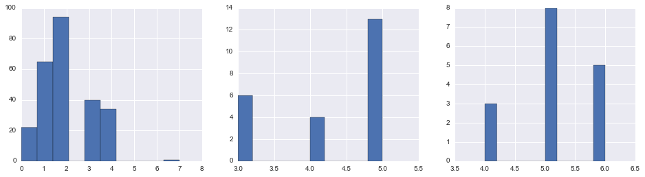
In [73]:
cabinclass_features = ['ImputedAge', 'EmbarkedEncoding', 'ImputedFare', 'Parch', 'PclassEncoding',
                       'SexEncoding', 'SibSp', 'TicketGroupEncoding']
In [74]:
union['ImputedCabinClass'] = union.CabinClassIn [75]:
params_cabinclass = {'n_estimators': [10, 20, 30]}

clf_cabinclass = sklearn.grid_search.GridSearchCV(sklearn.ensemble.RandomForestClassifier(), params_cabinclass)
clf_cabinclass.fit(union[cabinclass_filter][cabinclass_features], union[cabinclass_filter].CabinClass)
/Users/Estinox/bin/anaconda3/lib/python3.5/site-packages/sklearn/cross_validation.py:516: Warning: The least populated class in y has only 1 members, which is too few. The minimum number of labels for any class cannot be less than n_folds=3.
% (min_labels, self.n_folds)), Warning)
GridSearchCV(cv=None, error_score='raise',
estimator=RandomForestClassifier(bootstrap=True, class_weight=None, criterion='gini',
max_depth=None, max_features='auto', max_leaf_nodes=None,
min_samples_leaf=1, min_samples_split=2,
min_weight_fraction_leaf=0.0, n_estimators=10, n_jobs=1,
oob_score=False, random_state=None, verbose=0,
warm_start=False),
fit_params={}, iid=True, n_jobs=1,
param_grid={'n_estimators': [10, 20, 30]}, pre_dispatch='2*n_jobs',
refit=True, scoring=None, verbose=0)
In [76]:
union.loc[~cabinclass_filter, 'ImputedCabinClass'] = clf_cabinclass.predict(union[~cabinclass_filter][cabinclass_features])In [77]:
encoder_list = ['ImputedCabinClass']
encoder = []

for i, e in enumerate(encoder_list):
    print(i,e)
    encoder.append(sklearn.preprocessing.LabelEncoder())
    union['{}Encoding'.format(e)] = union[e]
    union.loc[~union[e].isnull(), '{}Encoding'.format(e)] = encoder[i].fit_transform(union[~union[e].isnull()][e])
0 ImputedCabinClass
In [78]:
fig, axes = plt.subplots(1, 3, figsize=(16,4))

for i, pclass in enumerate(np.sort(union.Pclass.unique())):
    union.loc[(union.Pclass == pclass), 'ImputedCabinClassEncoding'].hist(ax=axes[i])
    union.loc[(union.Pclass == pclass), 'CabinClassEncoding'].hist(ax=axes[i])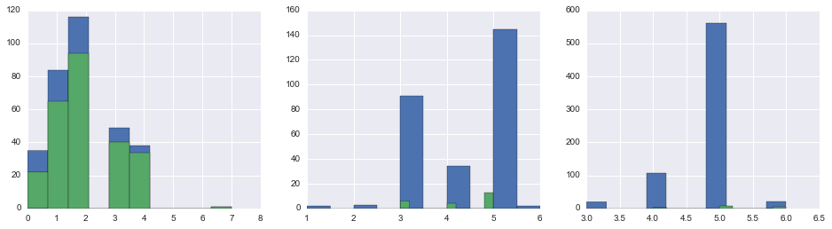
Cabin Number
Trying to be a creative here. My hypothesis is that the cabin numbers are laid out either from the front to the back, so the number would indicate whether if the room is at the front, middle, or the back of the ship.
In [79]:
def cabin_number_extract(x):
    if len(x) <= 1:
        return np.NAN

    for cabin in x.split(' '):
        if len(cabin) <= 1:
            continue
        else:
            return cabin[1:]
    return np.NAN

union.loc[~union.Cabin.isnull(), 'CabinNumber'] = union.Cabin[~union.Cabin.isnull()].apply(cabin_number_extract)
In [80]:
union[cabinclass_filter][['CabinNumber', 'Cabin']].head()| CabinNumber | Cabin | |
|---|---|---|
| 1 | 85 | C85 |
| 3 | 123 | C123 |
| 6 | 46 | E46 |
| 10 | 6 | G6 |
| 11 | 103 | C103 |
In [81]:
features_cabinnumber = ['ImputedAge', 'ImputedCabinClassEncoding', 'EmbarkedEncoding', 'ImputedFare', 'Parch',
                        'PclassEncoding', 'SibSp', 'SexEncoding', 'FamilySize', 'Alone', 'TitleEncoding',
                        'FamilyNameEncoding', 'TicketGroupEncoding', 'Mother']
In [82]:
encoder_list = ['CabinNumber']
encoder = []

for i, e in enumerate(encoder_list):
    print(i,e)
    encoder.append(sklearn.preprocessing.LabelEncoder())
    union['{}Encoding'.format(e)] = union[e]
    union.loc[~union[e].isnull(), '{}Encoding'.format(e)] = encoder[i].fit_transform(union[~union[e].isnull()][e])
0 CabinNumber
In [83]:
union['ImputedCabinNumber'] = union.CabinNumberEncodingIn [84]:
params_cabinnumber = {'n_estimators': [10, 20, 50, 100]}
clf_cabinnumber = sklearn.grid_search.GridSearchCV(sklearn.ensemble.RandomForestClassifier(), params_cabinnumber)

#clf_cabinnumber = sklearn.neighbors.KNeighborsClassifier(n_neighbors=5)

clf_cabinnumber.fit(union[~union.CabinNumber.isnull()][features_cabinnumber], union[~union.CabinNumber.isnull()].CabinNumberEncoding.astype(int))
/Users/Estinox/bin/anaconda3/lib/python3.5/site-packages/sklearn/cross_validation.py:516: Warning: The least populated class in y has only 1 members, which is too few. The minimum number of labels for any class cannot be less than n_folds=3.
% (min_labels, self.n_folds)), Warning)
GridSearchCV(cv=None, error_score='raise',
estimator=RandomForestClassifier(bootstrap=True, class_weight=None, criterion='gini',
max_depth=None, max_features='auto', max_leaf_nodes=None,
min_samples_leaf=1, min_samples_split=2,
min_weight_fraction_leaf=0.0, n_estimators=10, n_jobs=1,
oob_score=False, random_state=None, verbose=0,
warm_start=False),
fit_params={}, iid=True, n_jobs=1,
param_grid={'n_estimators': [10, 20, 50, 100]},
pre_dispatch='2*n_jobs', refit=True, scoring=None, verbose=0)
In [85]:
union.loc[union.CabinNumber.isnull(), 'ImputedCabinNumber'] = clf_cabinnumber.predict(union[union.CabinNumber.isnull()][features_cabinnumber])In [86]:
encoder_list = ['ImputedCabinNumber']
encoder = []

for i, e in enumerate(encoder_list):
    print(i,e)
    encoder.append(sklearn.preprocessing.LabelEncoder())
    union['{}Encoding'.format(e)] = union[e]
    union.loc[~union[e].isnull(), '{}Encoding'.format(e)] = encoder[i].fit_transform(union[~union[e].isnull()][e])
0 ImputedCabinNumber
In [87]:
union[cabinclass_filter][['CabinNumber']].describe()| CabinNumber | |
|---|---|
| count | 289 |
| unique | 104 |
| top | 6 |
| freq | 9 |
In [88]:
fig, ax = plt.subplots(figsize=(16,4))

union.ImputedCabinNumberEncoding.hist(ax=ax)
union.CabinNumberEncoding.hist(ax=ax)
<matplotlib.axes._subplots.AxesSubplot at 0x11ab93a58>
Cabin N-Tile
Take a look at the min and max of our cabins
In [89]:
union.loc[~union.CabinNumber.isnull(), 'CabinNumber'] = union[~union.CabinNumber.isnull()].CabinNumber.astype(int)In [90]:
union.CabinNumber.min(), union.CabinNumber.max()(2, 148)
In [91]:
def cabin_tile(x):
    if x == np.NAN:
        return np.NAN

    if x <= 50:
        return 0
    elif x <= 100:
        return 1
    else:
        return 2

union['CabinTertile'] = union.CabinNumber
union.loc[~union.CabinTertile.isnull(), 'CabinTertile'] = union.CabinTertile[~union.CabinTertile.isnull()].apply(cabin_tile)
union['ImputedCabinTertile'] = union.CabinTertile
In [92]:
params_cabinnumber = {'n_estimators': [10, 20, 50, 100]}
clf_cabinnumber = sklearn.grid_search.GridSearchCV(sklearn.ensemble.RandomForestClassifier(), params_cabinnumber)

clf_cabinnumber = sklearn.neighbors.KNeighborsClassifier(n_neighbors=5)

clf_cabinnumber.fit(union[~union.CabinTertile.isnull()][features_cabinnumber], union[~union.CabinTertile.isnull()].CabinTertile.astype(int))
KNeighborsClassifier(algorithm='auto', leaf_size=30, metric='minkowski',
metric_params=None, n_jobs=1, n_neighbors=5, p=2,
weights='uniform')
In [93]:
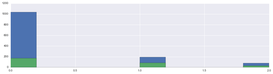
union.loc[union.CabinTertile.isnull(), 'ImputedCabinTertile'] = clf_cabinnumber.predict(union[union.CabinTertile.isnull()][features_cabinnumber])In [94]:
fig, ax = plt.subplots(figsize=(16,4))

union.ImputedCabinTertile.hist(ax=ax)
union.CabinTertile.hist(ax=ax)
<matplotlib.axes._subplots.AxesSubplot at 0x11cab7b38>
Model Fitting
Base Line
If we just predicted everyone to not surive, then we’d have 61.6% accuracy rate. So this is the minimum base life we have to beat with our classifier.
In [95]:
len(union[union.Survived == 0]) / len(union[~union.Survived.isnull()])0.6161616161616161
Null Checks
In [96]:
features = ['EmbarkedEncoding', 'Parch', 'PclassEncoding', 'SexEncoding', 'SibSp', 'TitleEncoding', 'FamilySize', 'Alone',
             'FamilyNameEncoding', 'ImputedAge', 'Mother', 'ImputedFare', 'TicketGroupEncoding', 'ImputedCabinTertile']
Check for null entries in our features
In [97]:
# Make sure that there are no Nan entries in our dataset
union[features][~union.Survived.isnull()][pd.isnull(union[features][~union.Survived.isnull()]).any(axis=1)]| EmbarkedEncoding | Parch | PclassEncoding | SexEncoding | SibSp | TitleEncoding | FamilySize | Alone | FamilyNameEncoding | ImputedAge | Mother | ImputedFare | TicketGroupEncoding | ImputedCabinTertile |
|---|
Okay, good, the above gave us no rows of null entries. We can continue.
Fitting
I’ve commented out a few classifiers I’ve tried to fit the model with. If you’ve cloned this note book, you can easily uncomment out thos rows and check out the results for yourselves.
For each classifier, I’ve decided to use grid search cross validation, and have the grid search return the best parameter with the best cross validation score.
In [98]:
params_c = {'C':[0.005, 0.1,0.5,1,2,5]}
params_n_estimators = {'n_estimators':[100, 500,1000,2000,4000]}

clfs = []
training_filter = ~union.Survived.isnull()

#clfs.append(sklearn.grid_search.GridSearchCV(sklearn.linear_model.LogisticRegression(), params_c, cv=5, scoring='f1'))
#clfs.append(sklearn.grid_search.GridSearchCV(sklearn.svm.SVC(), params_c, cv=5, n_jobs=4))
clfs.append(sklearn.grid_search.GridSearchCV(sklearn.ensemble.RandomForestClassifier(), params_n_estimators, cv=5, n_jobs=4))
#clfs.append(sklearn.grid_search.GridSearchCV(sklearn.ensemble.AdaBoostClassifier(), params_n_estimators, cv=5, n_jobs=4))
#clfs.append(sklearn.naive_bayes.GaussianNB())

for clf in clfs:
    clf.fit(union[training_filter][features], union[training_filter].Survived)

print('models fitted')
models fitted
In [99]:
for clf in clfs:
    if isinstance(clf, sklearn.grid_search.GridSearchCV):
        print(clf.best_estimator_)
        print(clf.best_params_)
        print(clf.best_score_)
        print(clf.grid_scores_)
        print('\n')
    #elif isinstance(clf, sklearn.naive_bayes.GaussianNB):
    else:
        print(clf)
RandomForestClassifier(bootstrap=True, class_weight=None, criterion='gini',
max_depth=None, max_features='auto', max_leaf_nodes=None,
min_samples_leaf=1, min_samples_split=2,
min_weight_fraction_leaf=0.0, n_estimators=1000, n_jobs=1,
oob_score=False, random_state=None, verbose=0,
warm_start=False)
{'n_estimators': 1000}
0.837261503928
[mean: 0.83277, std: 0.01839, params: {'n_estimators': 100}, mean: 0.83614, std: 0.02583, params: {'n_estimators': 500}, mean: 0.83726, std: 0.02555, params: {'n_estimators': 1000}, mean: 0.83502, std: 0.02497, params: {'n_estimators': 2000}, mean: 0.83502, std: 0.02683, params: {'n_estimators': 4000}]
How well have we trained against our own training set.
In [100]:
for clf in clfs:
    y_train_pred = clf.predict(union[training_filter][features])
    print(type(clf.best_estimator_) if isinstance(clf, sklearn.grid_search.GridSearchCV) else type(clf))
    print(sklearn.metrics.classification_report(y_train_pred, union[training_filter].Survived))
<class 'sklearn.ensemble.forest.RandomForestClassifier'>
precision recall f1-score support
0.0 1.00 1.00 1.00 550
1.0 1.00 1.00 1.00 341
avg / total 1.00 1.00 1.00 891
How important were each of the features in our random forest?
In [101]:
for clf in clfs:
    if isinstance(clf, sklearn.grid_search.GridSearchCV):
        if isinstance(clf.best_estimator_, sklearn.ensemble.forest.RandomForestClassifier):
            print('Random Forest:')
            print(pd.DataFrame(list(zip(clf.best_estimator_.feature_importances_, features))
                               , columns=['Importance', 'Feature']).sort_values('Importance', ascending=False))
Random Forest:
Importance Feature
3 0.168709 SexEncoding
11 0.161194 ImputedFare
8 0.157862 FamilyNameEncoding
9 0.143067 ImputedAge
5 0.114327 TitleEncoding
2 0.069930 PclassEncoding
6 0.039600 FamilySize
12 0.034325 TicketGroupEncoding
4 0.027307 SibSp
0 0.025159 EmbarkedEncoding
13 0.024457 ImputedCabinTertile
1 0.016596 Parch
7 0.009526 Alone
10 0.007940 Mother
How certain we are of our predictions? We can graph it out using predict proba.
In [102]:
for clf in clfs:
    if callable(getattr(clf, 'predict_proba', None)):
        pd.Series(clf.predict_proba(union[training_filter][features])[:,0]).hist()
        plt.title('Probability of Our Suvival Confidence')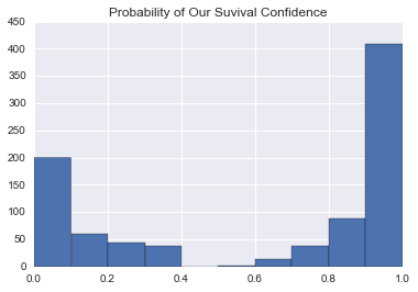
Submission
Finally, we’ll loop through all our classifiers and save the predicted csv file.
In [103]:
final_submission = []
for i, clf in enumerate(clfs):
    final_submission.append(union[~training_filter].copy())
    final_submission[i]['Survived'] = pd.DataFrame(clf.predict(union[~training_filter][features]))
    name = clf.best_estimator_.__class__.__name__ if isinstance(clf, sklearn.grid_search.GridSearchCV) else clf.__class__.__name__

    final_submission[i].Survived = final_submission[i].Survived.astype(int)
    final_submission[i].to_csv('titanic_{}.csv'.format(name), columns=['PassengerId', 'Survived'], index=False)
Extras
Over here, we have the learning curve analysis from Andrew Ng’s machine learning class.
In [104]:
from sklearn import learning_curve
def plot_learning_curve(estimator, title, X, y, ylim=None, cv=None,
                        n_jobs=1, train_sizes=np.linspace(.1, 1.0, 5)):
    """
    Generate a simple plot of the test and traning learning curve.

    Parameters
    ----------
    estimator : object type that implements the "fit" and "predict" methods
        An object of that type which is cloned for each validation.

    title : string
        Title for the chart.

    X : array-like, shape (n_samples, n_features)
        Training vector, where n_samples is the number of samples and
        n_features is the number of features.

    y : array-like, shape (n_samples) or (n_samples, n_features), optional
        Target relative to X for classification or regression;
        None for unsupervised learning.

    ylim : tuple, shape (ymin, ymax), optional
        Defines minimum and maximum yvalues plotted.

    cv : integer, cross-validation generator, optional
        If an integer is passed, it is the number of folds (defaults to 3).
        Specific cross-validation objects can be passed, see
        sklearn.cross_validation module for the list of possible objects

    n_jobs : integer, optional
        Number of jobs to run in parallel (default 1).
    """
    plt.figure()
    plt.title(title)
    if ylim is not None:
        plt.ylim(*ylim)
    plt.xlabel("Training examples")
    plt.ylabel("Score")
    train_sizes, train_scores, test_scores = learning_curve(
        estimator, X, y, cv=cv, n_jobs=n_jobs, train_sizes=train_sizes)
    train_scores_mean = np.mean(train_scores, axis=1)
    train_scores_std = np.std(train_scores, axis=1)
    test_scores_mean = np.mean(test_scores, axis=1)
    test_scores_std = np.std(test_scores, axis=1)
    plt.grid()

    plt.fill_between(train_sizes, train_scores_mean - train_scores_std,
                     train_scores_mean + train_scores_std, alpha=0.1,
                     color="r")
    plt.fill_between(train_sizes, test_scores_mean - test_scores_std,
                     test_scores_mean + test_scores_std, alpha=0.1, color="g")
    plt.plot(train_sizes, train_scores_mean, 'o-', color="r",
             label="Training score")
    plt.plot(train_sizes, test_scores_mean, 'o-', color="g",
             label="Cross-validation score")

    plt.legend(loc="best")
    return plt

#for clf in clfs:
#    name = clf.best_estimator_.__class__.__name__ if isinstance(clf, sklearn.grid_search.GridSearchCV) else clf.__class__.__name__
#    plot_learning_curve(clf, name, union[training_filter][features], union[training_filter].Survived, train_sizes=np.linspace(0.3,1,5))
Conclusion
Was definitely fun developing this notebook, and hopefully it has helped anyone who’s trying to tackle the Kaggle Titanic problem. And again, if you’re looking for the source of the Jupyter notebook, it can be found in the introduction. Thanks for reading!